In past chapters, we have devoted much time to presenting exponential functions. We found that it is related to the following differential equation: $$ f'(x) = k\cdot f(x) \,,$$
that has solutions in the shape of $$f(x) = C\cdot e^{kx} \,,$$
where $C$ and $k$ are some constants. In fact, we could define the $e^x$ function as a function solving this kind of equation, so much is the exponential and its equation is related. Let's see where this differential equation stands out. We'll also look at another way of constructing differential equations using differentials and Leibniz notation.
Why devote one comprehensive chapter to one differential equation? Indeed, there are an infinite number of possible differential equations that have many solutions. But it turns out that only certain shapes of differential equations exist in nature. Explaining this by hard mathematics requires a knowledge of very advanced differential geometry. But we get a better understanding if we look at the individual examples of differential equations and feel them out, which is the aim of this chapter.
At a driving school, they want students to drive very safely. They often tell novice motorists how dangerous corners are that you can't see behind. A common maxim is, go to the bend fast enough so that if your brakes break, you can reach it in 2 seconds at any time. But what does such a ride really look like? So we're driving at some $v(t)$ speed in the car, there's always some distance $s(t)$ (it changes in time) ahead of us into the turn, and it has to be true that at any given moment $v(t) \cdot T = s(t)$ for $T=2\,\mathrm s$, which corresponds to the fact that at $v(t)$ time, $T$ would cover exactly the distance s(t)$ left into the turn.
Anyway, acceleration is a derivative of speed by time.
Fortunately, we know one important thing: speed is the derivative of distance by time. Why? We can know the average speed as $v_p = s_c/t_c$, or the average distance traveled for the total time. We can write more accurately that $v_p = (s_c(t_0 + t_c) - s_c (t_0)/t_c$, where the distance traveled is the difference in distance at the end of the action and distance at the beginning of the action. The wise ones can already see that you just do a limit transition of $t_c \to 0$ and you get that speed is a derivative of position by time. In other words, instantaneous velocity is the average velocity over an infinitesimal time.
$$ s'(t) T = s(t) \Rightarrow s'(t) = s(t) \cdot \frac{-1}{T} \,. $$
Now we don't have to say anything anymore because we got a known differential equation that leads to an exponential solution. We see that $f(x)$ equals $s(t)$ and $k$ equals $1/T$. So we might as well write that $$s(t) = C \cdot e^{-t/T}\,.$$
This means that the distance travelled decreases exponentially over time. Let's say $s(0)$ is 100 meters so we can see what the function looks like. Then necessarily $C=s(0)$ and we can bring the function to the chart below.
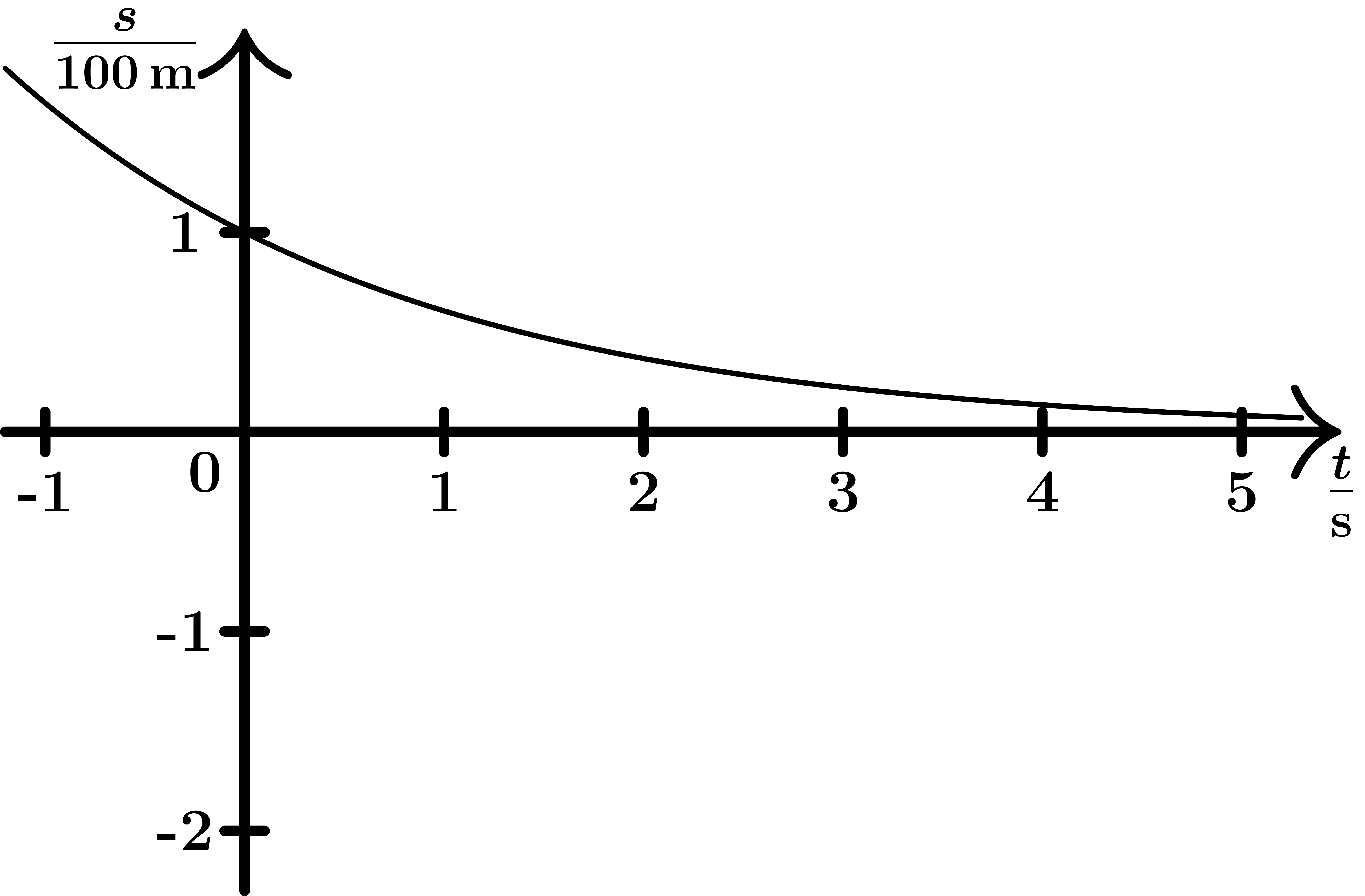
Negative times mean we're assuming the car went the same way some time ago $t=0$ and we're looking at where it was before the measurements started. Since the exponential argument is negative (we have $e^{-t}$, but we were used to $e^t$), the function drops rapidly instead of rising rapidly. But the exponential character is preserved, think that replacing $t$ with $-t$ only the graph has mirrored the $y$ axis.
We solved the problem above using Newton's notation. Another option is to write the equation in Leibniz notation: $$ \frac{\mathrm{d} s}{\mathrm{d} t} = -s(t) \frac{1}{T} \,. $$
We would like to integrate this equation somehow to get from differentials to normal quantities. But we can only do integration if there are only expressions on each side of the equation that depend on the quantity we integrate. So we multiply the equation by $\mathrm d t$ and divide by $s(t)$, then integrate: $$\begin{align*} \frac{1}{s(t)} \mathrm{d} s&= - \frac{1}{T} \mathrm{d} t\\ \int_{s_0}^{s} \frac{1}{s(t)} \mathrm{d} s&= \int_{t_0}^t - \frac{1}{T} \mathrm{d} t\,. \end{align*}$$
We can do the integration if we remember that the derivative of $\log (x)$ is $1/x$. The left-hand integral can thus be easily quantified: $$\begin{align*} \int_{s_0}^{s} \frac{1}{s(t)} \mathrm{d} s&= \int_{t_0}^t - \frac{1}{T} \mathrm{d} t\\ \left[ \log (s) \right]_{s_0}^s&= - \frac{1}{T} (t -t_0)\\ \log \left( \frac{s}{s_0}\right)& = - \frac{1}{T} (t -t_0)\\ s & = s_0 e^{- \frac{1}{T} (t -t_0)}\,. \end{align*}$$
On the last line, we put both sides of the equation into the exponential. Since this is the inverse of the logarithm, we got a result that is the same as the Newton notation (we just have to think $t_0=0$).
Perhaps in every school role there is talk of not neglecting air resistance for simplicity. But what is a plot in which this resistance is not neglected? Here we can no longer do without Newton's Law of Force. This law, which is taught to every schoolboy as early as primary school, states that there is the following relationship between the force exerted on a body, its mass and the acceleration granted: $$ F= m\cdot a \,.$$
Movement with air resistance takes place, for example, so that we have some kind of body that has resistance forces on it as it moves. This resistance force is greater the faster our body is (because the faster it hits the air and the more it brakes). One possible form of resistance force is e.g.: $$ F_o = - k\cdot v \,.$$
The minus sign indicates that it is acting against the direction of motion, further it is directly proportional to the speed. So let's look, for example, at a maglev that at the beginning is going at some speed and only the resistance force is acting on it. If we put a single acting force of $F=F_O$ in Newton's Law, we get this differential equation: $$\begin{align*} -k \cdot v &= m \cdot v'(t) \\ v'(t) &= - \frac{k}{m} \cdot v \,. \end{align*}$$
The solution to the equation is now clear because this is our known exponential differential equation. So we get: $$ v(t) = v_0 \cdot e^{-k/m \cdot t} \,,$$
where $v_0$ is the speed at the beginning. So the velocity drops much like the graph above. According to our model, it will never go further than zero. Using differentials, we would solve the equation similarly to the previous equation for safe driving.
Everybody knows that today's space rockets contain a lot of fuel, even 80% of the mass of the entire rocket. This fuel fires the rocket, creating the same force that buoys it. We know from Newton's Second Law that a body at the same acting force accelerates more the lighter it is. But burning fuel in flight reduces the rocket's mass. So what is the course of the rocket's speed through time? Let's write the second Newton first, but in a more general way: $$\begin{align*} F = \frac{\mathrm{d} p}{\mathrm{d} t} = m(t) \cdot v'(t) + m'(t) v(t) \,. \end{align*}$$
As another prediction to simplify the calculation, imagine that the rocket has already ascended into orbit and is thus beyond the influence of gravity. So it pays $F=0$. Next, two options are opening up before us: address the dependencies of time, or address the dependence of the change in rocket speed on the jettisoned mass of fuel. First, let's look at the first one.
$$\begin{align*} m(t) v'(t) &= - M v_e \\ (m_0-Mt) v'(t) &= - M v_e \\ v'(t) &= - \frac{Mv_e}{(m_0-Mt)} \\ \int v'(t) \,\mathrm{d} t &= -\int \frac{Mv_e}{(m_0-Mt)} \,\mathrm{d} t\,. \end{align*}$$
The intelligence on the right side may be familiar, we have encountered it in the case of four dogs chasing each other in a circle. The logarithm comes out of it, because $$\begin{align*} \frac{\mathrm{d}}{\mathrm{d}t} v_e \log (m_0 - Mt) = v_e\frac{\mathrm{d}\log (m_0 - Mt)}{\mathrm{d}m_0-Mt} \cdot \frac{\mathrm{d}(m_0 - Mt)}{\mathrm{d}t}= \frac{-M\cdot v_e}{m_0-Mt} \,. \end{align*}$$
So this result can be used to continue our equation: $$\begin{align*} \int v'(t) \,\mathrm{d} t &= -\int \frac{Mv_e}{(m_0-Mt)} \,\mathrm{d} t\,. \\ v(t) &= v_e \log (m_0 - Mt) +C \,. \end{align*}$$
We can set the constant so that the rocket's speed at time $t=0$ is zero, so $C= -v_e \log(m_0)$: $$ v(t) = v_e \log \left( \frac{m_0 - Mt}{m_0}\right) \,.$$
So for a speed solution, let's assume that mass is a function of speed. This gives us the following equation: $$\begin{align*} m(v) v' + m' v_e &= 0 \\ m(v) v' &= -m' v_e \,. \end{align*}$$
We want to ideally construct a differential equation in the $v$ variable, however we see two time derivatives here. That's not appropriate, we'd like to have a rate derivative. Therefore, we can use the identity presented in the second chapter on the ratio of two derivatives: $$\begin{align*} \frac{m(v)}{v_e} &= -\frac{m'}{v'} \\ \frac{m(v)}{v_e} &= -\frac{\frac{\mathrm{d} m}{\mathrm{d}t} }{\frac{\mathrm{d} v}{\mathrm{d}t}} \\ -\frac{m(v)}{v_e} &= \frac{\mathrm{d} m}{\mathrm{d}v} \,. \end{align*}$$
$$\begin{align*} m'(v) = \frac{m(v)}{v_e} \Rightarrow m(v) &= C\cdot e^{-v/v_e} \\ m(v) &= m_0 e^{-v/v_e} \,. \end{align*}$$
We chose the $C$ constant so that at the beginning of the plot the rocket would have a mass of $m_0$. We see that we have arrived at an equivalent equation to the time case.
Everybody knows that as we go up, the air pressure goes down. At Mt. Everest is even boiling water at about 70 degrees Celsius. But how exactly does this descent happen? To do this, we need a hydrostatic equation: $$\begin{align*} p = h\rho g \,. \end{align*}$$
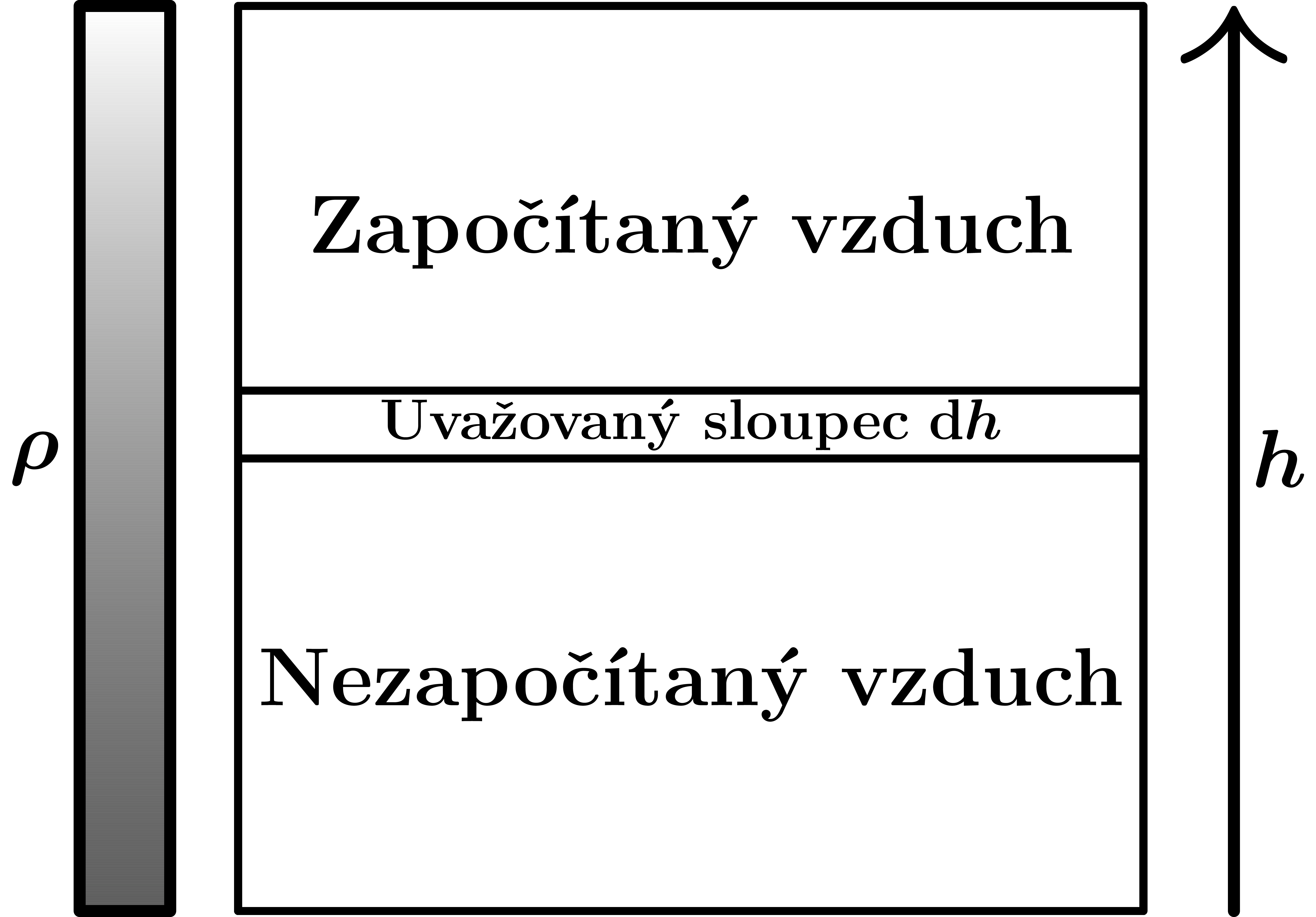
This equation describes the pressure of $p$, which causes a column of fluid with a density of $\rho$ and a height of $h$ at gravitational acceleration of $g$. We cannot use it directly for air, as air density decreases with the ambient pressure of $p$ (the more compressed the less dense the air). Air density can be described using the so-called ideal gas state equation. Since atmospheric models are mostly more complicated than our estimate anyway, consider the example of air having the same temperature everywhere. Then the state equation for air has the following shape: $$ p \cdot V = nR T = k_1\,,$$
where we marked the members on the right-hand side as the constant $k_1$ (indeed, the right-hand side is constant for constant temperature in our case). From the status equation, we get $p = k_1/V$. This means that the volume of a certain mass of air shrinks with the pressure. We know further that the density is inversely proportional to the volume of air: $\rho = m /V$. So we can briefly write $p = k \rho$, where $k$ is some other constant (we could determine it, but it would take too much time). We can combine this finding with knowledge of the hydrostatic equation. Because we can imagine the atmosphere as a lot of very thin layers of air, with each layer having an immutable density. So let's say that so far we've factored in the pressure an air column the size of $h$ and we want to add the aforementioned small column the height of $\mathrm d h$. Everything is drawn in the figure below.
We get the following equation: $$\begin{align*} p(h + \mathrm d h) \doteq p(h) + \mathrm d h \cdot p'(h) &= p(h) + \rho(p) g \mathrm d h \\ p'(h) &= \rho(p) g \\ p'(h) &= k_1 p g \,. \end{align*}$$
We already know this equation, so we might as well write a solution: $$\begin{align*} p(h) &= p_0 \cdot e^{k_1g h} \,. \end{align*}$$
We see that the pressure increases exponentially as the $h$ increases. This also means that if, for example, we climb a mountain and go down, the pressure goes down exponentially.
Some elements of the periodic table break up into other elements in a certain configuration. But this disintegration does not happen all at once, but gradually and so-called stochastically. That means that at any given moment, every nucleus has a chance to break apart. We operate with the term half-life of $T$, which is the time for which each core has a chance to break up 50%. For example, the Thorium element $^{234}\mathrm{Th}$ has a half-life of $24{,}10$ days.
$$\begin{align*} N'(t) &= -\lambda N(t) \,. \end{align*}$$
There is a minus in the equation, since the number of particles is, of course, dwindling. We may as well solve this equation because it is a sample exponential equation from the beginning of the chapter: $$\begin{align*} N(t) &= N_0 e^{-\lambda t} \,. \end{align*}$$
We marked the integration constant $N_0$ as the initial number of particles. We can further determine what the relationship is between $\lambda$ and $T$. Just look at our equation and put the number of particles at half and $t=T$. $$\begin{align*} N(T) &= N_0/2 \\ N_0 e^{-\lambda T} &= N_0/2 \\ e^{-\lambda T} &= 1/2 \\ \lambda T &= -\log (1/2) \\ T &= \frac{\log (2)}{\lambda} \,. \end{align*}$$
We used the minus from the equation to invert the value inside the logarithm according to the rule $a \log (b) = \log (a^b)$ and $a=-1$. So we got a translation relationship between $T$ and $\lambda$, so we know the course of radioactive decay -- it's exponential.
If you've ever been to the harbor, you've seen boatswain tie boats to the shore with a rope on a special bollard. However, the reeling of the rope will be met at other times in shipbuilding work, e.g. when we want to pull (return) the anchor from the water. But let us concentrate on the bollard on the pier, for it is easier to imagine. The question is: what is the frictional force of the rope depending on the angle of the rope's tangle on the bollard?
Let's first remember how the friction force actually works. Let's imagine an object on a flat surface: like a book on a table. We're introducing a coefficient of friction between the table and the $f$ book. The book further exerts a normal $N$ force on the table (due to gravity) and we can push it forward with the force of $F$. In this case, the friction force is counteracting the direction of motion and has a size of $T = Nf$. So the friction force is proportional to the normal force of $N$, which you can try yourself at home-you can push the book from the top of your hand, and the more you push, the more resistance there will be to moving.
In our case, we wrap the rope around the bollard. Friction power here won't be as simple as with a book, because it acts on a curved surface. So we need to analyse the situation in more detail. Consider that there is a larger force of $F_1$ on one side of the curb and a smaller force of $F_0$ on the other end. In an equilibrium position just before the rope slides off the curb, the friction force of $T_{\mathrm{max}}$ is still exerted. He's definitely paying $F_1 = F_0 + T_{\mathrm{max}}$ (in the direction of the rope). However, the friction force is rather complicated, as it gradually increases with the filming of the rope. Let's draw a picture for a better understanding.
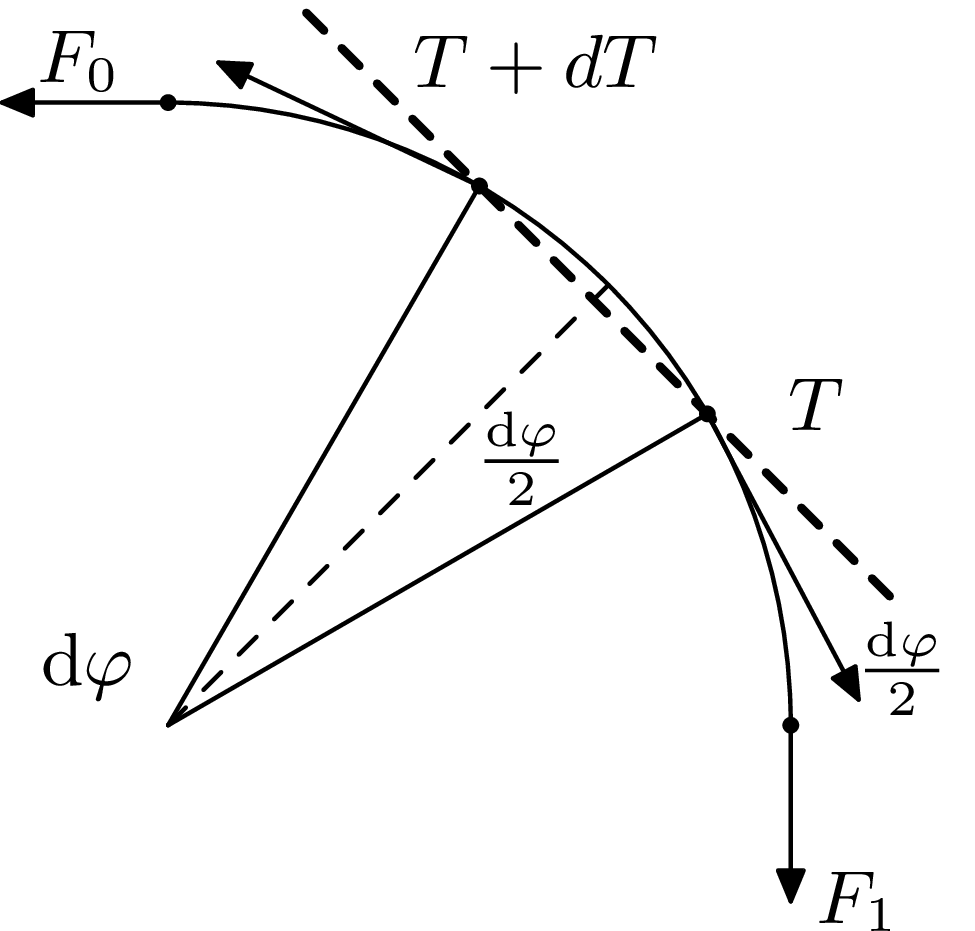
On this sketch, the thinner dashed line is the $\mathrm{d} \varphi$. Arrows coming from the ends of the angle are friction forces of sizes $T$ and $T+\mathrm{d} T$: over the angle of $\mathrm{d} \varphi$ to the strength of $T$, it adds a contribution of $\mathrm{d} T$ due to the friction force. The thicker dashed line is perpendicular to the thinner one, forming an angle of $\mathrm{d} \varphi/2$ with forces. You can verify this by turning the $T$ strength $90^\circ$. In the diagram, we drew the angle $\mathrm{d} \varphi$ to go see, but actually let's choose this angle very small.
Next, we can ask where normal power comes from: it's because of the voltage strength of $T$ and $T +\mathrm{d}T$. This force does not operate perpendicularly to the surface; a part of it acts directly as a normal force. We can draw the following triangle:
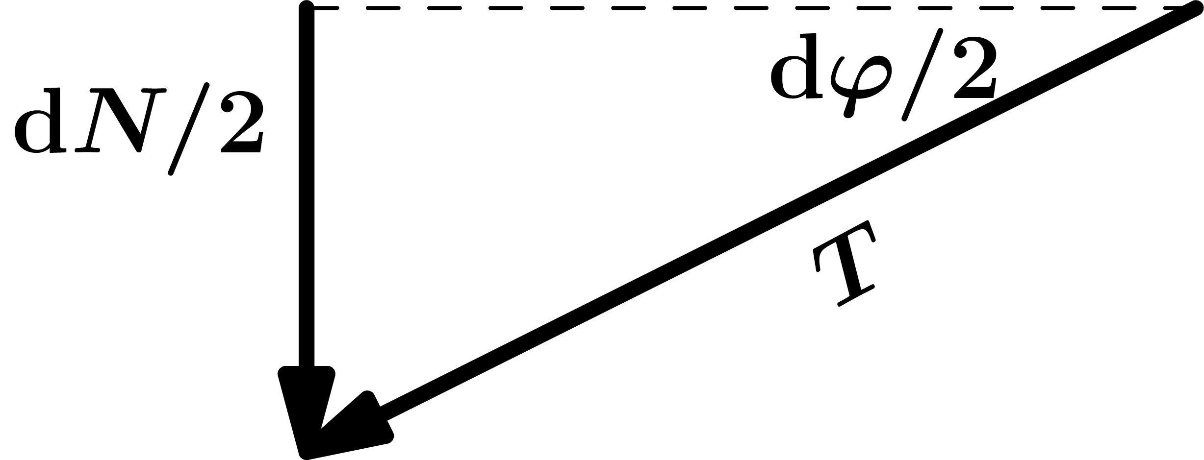
We could draw a similar triangle for $T+\mathrm{d} T$. Of course, the sketch is exorbitant, since $\mathrm{d} N$ should be very small, as should $\mathrm{d} \varphi$. Here, however, we can see that $$\begin{align*} \sin (\mathrm{d} \varphi/2) &= \frac{\mathrm{d}N/2}{T} \\ T\sin (\mathrm{d} \varphi) &= \mathrm{d}N \\ T &= \frac{\mathrm{d}N}{\sin (\mathrm{d} \varphi)} \,. \end{align*}$$
We're still going to express the $N$ we don't know using $T$, because these two variables are linked by friction: $$ \mathrm{d} N = \mathrm{d} T /f \Rightarrow Tf = \frac{\mathrm{d}T}{\sin (\mathrm{d} \varphi)} \,. $$
Of course, we'll do the limit crossing on the other side of the straight, but there's only $Tf$.
Here on the right-hand side of the resulting equation, we do a certain limit transition. We're doing it because we want to get some differential equation, so we would want to get some derivative into the equation. Let's make the limit transition so that $\mathrm{d} \varphi$ goes to zero, as we indicated at the beginning, it will look like this: $$\begin{align*} &\lim_{\mathrm{d} \varphi \to 0} \frac{\mathrm{d}T}{\sin (\mathrm{d} \varphi)} = \lim_{\mathrm{d} \varphi \to 0} \frac{\mathrm{d}T}{\frac{\sin (\mathrm{d} \varphi)}{\mathrm{d}\varphi}\mathrm{d}\varphi} = \lim_{\mathrm{d} \varphi \to 0} \frac{\mathrm{d}T}{\mathrm{d} \varphi} = \lim_{\mathrm{d} \varphi \to 0} \frac{(T + \mathrm{d}T) - T}{\mathrm{d} \varphi} \\ &= \lim_{\mathrm{d} \varphi \to 0} \frac{T(\varphi +\mathrm{d} \varphi) - T(\varphi)}{\mathrm{d} \varphi} = T'(\varphi) \,. \end{align*}$$
In this, we used that $$ \lim_{x\to 0} \frac{\sin (x) }{x} = 1 \,,$$
Which we mentioned in the derivative appendix of animated geometry. So hopefully you can see that by the limit transition we could get to the derivative. It's worth adding that this explanation of the derivative may be too comprehensive, for a standard physicist to see the expression $\mathrm{d} T/ \mathrm{d} \varphi$ and immediately conclude, without thinking, that this is a derivative of $T$. But such thinking comes from the fact that we take $\mathrm{d} T$ as differentials, which is not justified-here we just took them as numbers, and we didn't formally introduce differentials at all.
Anyway, after long periods, we finally got our differential equation: $$\begin{align*} T'(\varphi) &= T(\varphi) f \,. \end{align*}$$
Wonder of a world, this is a known exponential equation, so we can solve it before you can say: $$\begin{align*} T_{\mathrm{max}}(\varphi) &= F_0 e^{f \varphi} \,. \end{align*}$$
We chose the integration constant as $F_0$, to make the equation work for $\varphi = 0$. The equation tells us that the maximum friction force we generate by wrapping is equal to the lesser force $F_0$ multiplied by a factor that exponentially depends on the angle of rotation. As a practical consequence, for each rotation, the angle is increased by $2\pi$, so the friction force is increased by $e^{2\pi f}$-times. If $f=1/(2\pi)$ is for simplicity, each rotation increases the $e$-fold. This means that two rotations means roughly ten times the amount of friction force! So the next time you wrap a rope around a bollard or a tree, you don't even have to tie it, just wrap it enough times.
Body cooling can also be described using differential equations. Let's imagine we have, for example, a hot tea at $T_0=80^{\circ}\,\mathrm C$, the ambient temperature being room $T_p = 20^{\circ}\,\mathrm C$. We know from our own experience that the temperature of the tea drops over time until it reaches ambient temperature, while the ambient temperature hardly changes. But how fast is the temperature dropping? According to the Fourier law of thermal conductivity, heat flow is the difference in cup temperatures and ambient temperature (or the greater the difference in temperature, the more heat flows). This can be written as follows ($\lambda$ is a Greek small lambda): $$\begin{align} q = \lambda \Delta T \,. \end{align}$$
Or the heat flow is equal to $\lambda$ times the temperature difference of the cup and the surroundings. At the same time, assuming a constant heat flow, it is true that $$\begin{align} \delta T = -q t \,, \end{align}$$
or that the change in cup temperature is equal to the product of $-q$ (heat drains) and time $t$. Unfortunately, however, $\Delta T$ depends on $\delta T$. We can solve this by re-writing the change in heat over a small period of time, during which we assume a constant $\Delta T$: $$\begin{align} T(t+ \mathrm d t) \doteq T(t) + \mathrm d t \cdot T'(t) &= T(t) - q \mathrm d t \\ \mathrm d t \cdot T'(t) &= - \lambda \Delta T \mathrm d t \\ T'(t) &= - \lambda \Delta T \,. \end{align}$$
Here we could also express the change in temperature as $-q\mathrm d t$, since in a very small time $\mathrm d t$, we assume that $\Delta T$ will hardly change, and thus that $q$ will remain constant (and the time $\mathrm d t$ can be chosen as small as possible).
$$\begin{align} \Delta T'(t) &= - \lambda \Delta T \,. \end{align}$$
We already know this equation, and we can write that $$\begin{align} \Delta T &= T_0 e^{-\lambda t} \,, \end{align}$$
where $T_0$ is an integrating constant in the meaning of the initial temperature. So we see that the cooling also happens exponentially.
The main principle of finance is investment. We'll put some $p$ into an investment, and in time we'll get our money back with a bonus for our efforts. Usually we get our money back percentage-wise. That means we have some interest rate of $k$, and we get our money back of $kp$. For example, an interest rate of $k=1{,}05$ means five percent interest. We can then put the money we made back into the same investment. That's called compound interest.
We can see what kind of money we'll have in time. Zero year $p$, first year $kp$, second year $k^2p$ etc. But in less than a year? To do that, we're going to have to build a differential equation again. We can make a similar argument to radioactive decay, which is that the change in the number of money should be proportionate to the current number of money at any given time. Written mathematically using the $\lambda$ proportionality constant: $$\begin{align*} p'(t) = \lambda p(t) \,. \end{align*}$$
This is a familiar story, we are writing a solution: $$\begin{align*} p(t) = p_0 e^{\lambda t} \,. \end{align*}$$
Again, $p_0$ is relevant to the number of money we have going on in the beginning. We also want to know the relationship between $\lambda$ and $k$. We substitute $t = T = 1 \,\mathrm{year}$, and we get: $$\begin{align*} p(T) &= kp_0 \\ p_0 e^{\lambda T} &= kp_0 \\ e^{\lambda T} &= k \\ T &= \frac{\log (k)}{\lambda} \,. \end{align*}$$
So we've come to the conclusion that compound interest behaves exponentially. No wonder, then, that investors who use them get rich quickly. On the other hand, if our investment took the money, for example, because of inflation, we would have $k<1$, e.g. $k=0{,}98$ for conventional 2% inflation. We would then get a decreasing exponential ($\lambda$ would be negative because $\log (k) < 0$).
Even electrical circuits follow differential equations. Understanding them helps us understand how common circuits work in electronic devices, or we can even build our own circuits. But before we get to the more complicated components, let's first refresh the basics of electrical circuits.
In an electrical circuit, an electrical current flows like water in a ditch. We have a base quantity of $Q$ called electric charge, which is further worked on in physics-e.g. an electron has a so-called elementary charge of $-e$. The electric current is then the flow of charges. So we introduce the quantity $I$ as the magnitude of the electric current and it is naturally defined by the charge derivative: $I\equiv \dot Q$. We also introduce a $U$ voltage, which we measure always between two points of the circumference and indicates the force of the charges between the two points. Ultimately, we define a $R$ resistance that expresses what resistance the bullets have on some path. For most electrical elements, Ohm's Law applies, which relates the voltage to the element, the current flowing through the element, and the resistance of the element: $$\begin{align*} U &= I \cdot R\,. \end{align*}$$
We can make an analogy with the flow of water to facilitate the understanding of electrical current. In it, we can imagine charge as volume of water, current as volume flow per second, voltage as height difference between two points (the bigger the better the water flows), and resistance is the inverted width of the channel (the greater the width, the faster the flow, the greater the inverted width, the slower the flow).
One sample circuit is shown in the figure below. It consists of a flashlight that delivers a voltage of $U$, plus one resistor that gives the circuit a resistance of $R$. What we know about this circuit is that the voltage on the resistor is supplied by the flashlight, so it's equal to $U$. So we can write Ohm's law for resistor to get the current: $U=IR\Rightarrow I = U/R$.

The capacitor is another electrical component that accumulates charge. Each capacitor has a capacity of $C$ and the relationship between the charge on the capacitor, the voltage and this capacity applies: $$Q = CU\,.$$
Now let's focus on a simple $RC$ circuit with a capacitor and resistor. His diagram is as follows:

Suppose the capacitor is charged to an initial charge of $Q_0$. Subsequently, the charge will be discharged, we just have to find out how. For the resistor, Ohm's law is $U_{\mathrm r}=IR$ and for the capacitor $U_{\mathrm c}=Q/C$. Next, we can break down the stream by definition as $I=\dot Q $. So we can build an equation with voltages on both elements. But this time the voltage on the resistor is minus the voltage on the capacitor. It's because $$\begin{align*} U_{\mathrm r} &= U_{\mathrm c}\\ -\frac{\mathrm{d} Q}{\mathrm{d} t} \cdot R &= Q/C\\ \dot Q &= -\frac{1}{CR}\, Q\,. \end{align*}$$
A negative sign appeared in the equation because the $Q$ loss on the capacitor means a $Q$ dwelling in the perimeter (and on the resistor). From this equation, you can see that the capacitor is discharged as follows: $$\begin{align*} Q(t) &= Q_0 e^{-t/RC} \,. \end{align*}$$
Another possible component of the electrical circuit is the $L$ inductance coil. This component creates a magnetic field when current flows through it. The tension on it can be described by the following equation $$\begin{align*} U &= - L \dot I\,. \end{align*}$$
Let's look at the current in the simple circuit with resistor and coil as in the figure below
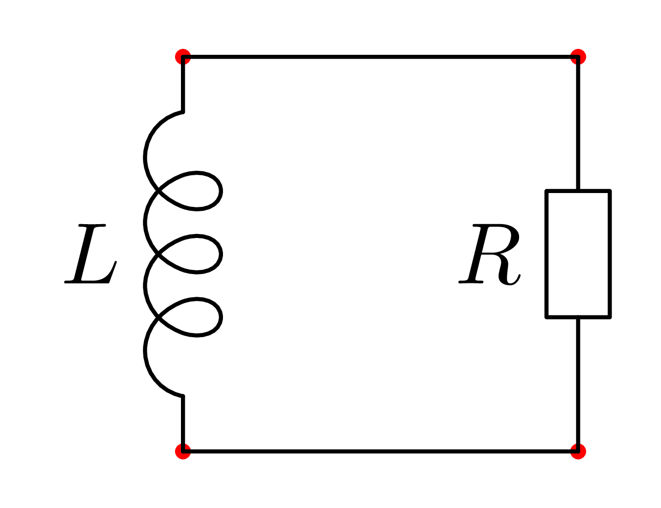
Once again, we construct an equation where the voltage on the coil equals the voltage on the resistor: $$\begin{align*} IR &= - L \dot I\\ \dot I &= -\frac{R}{L} I\,. \end{align*}$$
We got an exponential equation again, which we'll solve briskly: $$\begin{align*} I(t) &= I_0 e^{-\frac{R}{L}\, t} \,. \end{align*}$$
We're seeing harmonic oscillations again, this time in an electric current.
 About
About Articles
 Tutorials
 External links
 About me