Asymptote is a powerful program that can be used to create professional-looking vector images, graphs, or sketches. This is a sort of newer version of the Metapost, which it closely resembles, only more direct to use. Using Asymptote (or Metapost), I created my sketches into a series of articles Alive Geometry. In the program you can draw 2D as well as 3D drawings, I'll just focus on 2D drawings.
Like LaTeX this is not a WYSIWIG program but a programming language. You draw pictures not with your mouse, but by telling the program what you want to get, and it creates it for you. The advantage of this is that you can draw accurate analytical curves such as the $y=\sqrt{x}$ graph, but also that you can recycle code you have already written, or use for loops to create advanced shapes and save time.
The aim of this guide is to give a very brief account of how the program is installed and how it can be used to draw basic objects and functions. If you're interested in the program, you can read more about its features in the manual or read the longer English tutorial.
Let's start with the hardest part - installing a program and writing a Hello World program. If you want to just try the program without installing, then you can try the online environment for Asymptote. To make pictures, we will need the following three things:
Asymptote has no graphical interface in the base. You install it and it stays in the background on your PC. When you need it, you'll call it, and it will create a picture, following your commands. Instead, we need a Texmaker to write these commands. It's going to be our graphical interface in which we write our picture, and then we look at it. The GhostScript program, it's just a kind of dependency that helps Asymptote work with pdf files.
In the installation I calculate that you are using the Windows 10 operating system, and that you have about 1GB of free disk space.
If you are using Linux, you can replace the installation steps with a single line to the terminal. For Ubuntu:
sudo apt-get install asymptote texmaker ghostscript
For Arch Linux:
sudo pacman -S asymptote texmaker ghostscript
Create a folder on your computer and a file named *hw.asy. Open this file in Texmaker. Type the following in the window:
settings.outformat = "pdf";
unitsize(1cm);

draw(unitsquare);
The first line tells us that we want to use the pdf format. This format is useful for letting you view the result in Texmaker. However, you can change it to, for example, png (but this will lose its vectors) or svg or eps. You may find that some things (like hatching) break for the svg format, so I recommend using pdf or eps. After all, it can easily insert itself into a .tex document.

Next, change the compiler to the Asymptote program as shown in the image next to the button with the arrow on top. Now when you click or press F1 on the arrow, the file will be compiled (translated) and you will see the result on the right side.
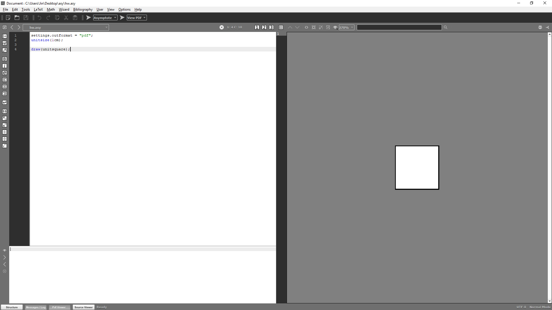
Using the command draw(unitsquare); we drew a square with an edge of one centimetre, and this is actually shown on the right side. The background of our image is white by default, so black four lines at the edge have been drawn. The image was then cut to the smallest possible size.
The asymptote language is similar to C or C++, e.g. comments are written identically using //. If you know their syntax, just skim the following section.
As in any language, we can set variables that have different data types, depending on what they represent (and how much space they take). Here is a brief overview:
int
real
pair
path
string
[]
Variables are good to declare first by writing the type of variable and its name. For example, if we write
int pocitadlo;
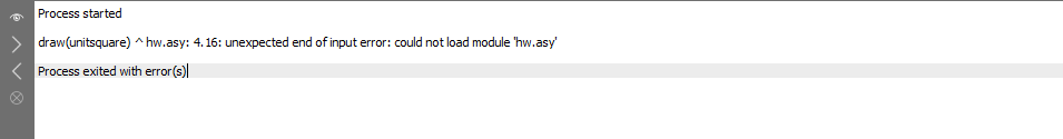
so we introduced an integer variable called sensation. A semicolon must be typed at the end of each command, otherwise Texmaker will throw up followed by an error message.
Variables can be given a value for example as follows:
int i,j;
i = 2;
j = i^2 + 2*4;
i = i + 1;
At the end of these lines, both and will equal 3 and j will equal 12. We've also defined multiple variables of the same type at once. You can also work with text strings:
string a;
int i;
i=1;
a = (string) i;
a = a + "23ctyri";
At the end of this example, and will contain the text string 1234.
It is worth noting that some variables are so-called system variables and change some parameters of the program. For example, the variable settings.outformat, which we met earlier, changes what output format we will have.
Functions are small programs within a program that we can define and then call to do some work for us. Typically still returns the output value. For example, we can define a function as follows:
real f(real x) {
 return x*2;
 }
This code says that the f takes one real parameter x and also returns a real parameter. We can call it as follows:
real y;
y = f(2.1);
Then the variable y will be equal to 4.2. There are still functions that do not return the parameter. We just call them, and they do something (like draw a line).
Another important thing will be the so-called for cycle. With it, we can do many things at once. For example:
int pocitadlo;
pocitadlo = 0;
for ( int i = 0; i <= 2 ; ++i){
 pocitadlo = pocitadlo + 1;
}
This cycle will execute an internal code for both and equal to zero, one and two, so eventually feeling will be equal to three.
Lines are drawn using the draw(path p). But first we need to know what the curve path and the point pair looks like. We can define a point by simply giving its coordinates (first $x$ coordinate, then $y$). However, it is useful to say in advance what units we work in (e.g. in centimetres). In total, we may have, for example, such a code:
unitsize(1cm);
pair z;
z = (1,0);
dot(z);
dot( (0,0) )
This will draw two dots at two different coordinates. We can define a curve as a path through some points, then we can draw it using the draw. It also depends on whether we want to connect the points directly or in a twist (using a B\u00e9zier curve). Direct link is done by -- and twisted link by .., as you can see in the following example;
unitsize(1cm);
path p1;
pair a;
a=(0,0);
p1 = a -- (1,1) -- (4,2) -- cycle;
draw(p1);
draw(a .. (1,-1) .. (4,-2) -- cycle);
Try what picture you get. The top is straight, while the bottom is seamlessly connected. By commanding cycle we go back to the beginning cyclically.
If you had written an extra fill(p1); in the previous one, the first curve would have been filled with black. The fill color can be changed (see manual p. 16).
You can still insert text into the image using the label( string name,pair posice). Of course name interprets LaTeX. So you just write, for example, just call the label( \$x^2$\(0.0)); and you get a nice $x^2$ in the beginning.
An example of all things shown is this code, which produces a numbered axis, you can extend it at any time:

settings.outformat = "pdf";
unitsize(1cm);

path osa;
real delka,prodl;

delka = 10;
prodl = 0.5;
osa = (-delka-prodl,0)--(delka+prodl,0);
draw(osa,Arrows );

path cara;
real rozpeti;

rozpeti = 0.2;

// Čáry do osy
for (int i = 0; i <= 2*delka ; ++i) {
 cara = (-delka+i,rozpeti) -- (-delka+i,-rozpeti);
 draw(cara);
 label((string) (i-delka),(-delka+i,-rozpeti*2 ));
}

for (int i = 0; i <= 2*delka*10 ; ++i) {
 if ( i % 10 != 0) {
 cara = (-delka+i/10,rozpeti/3) -- (-delka+i/10,-rozpeti/3);
 draw(cara);
 }
}
You can also load so-called modules (or libraries, packages) into the asymptote, which are extensions of program features written by someone else. One such package is called graph and allows us to draw graphs of functions.
settings.outformat="pdf";
unitsize(1cm);

import graph;

real f(real x) {
 return sqrt(x) + cos(pi/x) + log(x);
}
path g = graph(f,0.01,2);
draw(g);
Here we have determined the curve g using the graph function. For more on features and how to make them more subtle, see the listed tutorial on p. 28th.
In Asymptote, you can draw advanced pictures in the way I outlined above. I hope you now have a framework understanding of how to draw such pictures. Explaining multiple functions, such as drawing geometric shapes or transforming, would already make this text too long and would be pointless in the first place: the necessary information can be found simply on the Internet or in the referenced tutorial and manual.
If you found the instructions useful, check out the other Instructions or some of my articles. I can recommend, for example. Reviving geometry, a simple introduction to differential calculus.
 About
About Articles
 Tutorials
 External links
 About me