For all of those who are already a little bit oriented on the importance of derivative, integration, and how they relate to each other, I will address more practical matters in this appendix. I'm going to derive the derivatives of a few basic functions, and these are going to produce some integrals (because integration is the inverse of the derivative). All the results are then summarised in a clear table. At the same time, you can use derivation to verify that you understand everything correctly. I'm also going to cover features I didn't cover in the previous series, so don't worry about it if you don't know them.
The linear function $f(x)=x$ is perhaps the most basic function anyone can think of, in a similarly basic way we can calculate its derivative: $$\frac{\mathrm{d}}{\mathrm{d}x} f(x) = \lim_{h\to 0} \frac{ f(x+h)-f(x)}{h} = \lim_{h\to 0} \frac{ x+h-x}{h} = \lim_{h\to 0} 1 = 1\,.$$
We've already covered the $f(x)=x^2$ function in the series with its derivative. So let's do it again: $$\frac{\mathrm{d}}{\mathrm{d}x} f(x) = \lim_{h\to 0} \frac{ f(x+h)-f(x)}{h} = \lim_{h\to 0} \frac{ (x+h)^2-x^2}{h} = \lim_{h\to 0} \frac{ 2xh + h^2}{h} = \lim_{h\to 0} 2x + h = 2x\,.$$
Now let's look at an example of $f(x)=x^n$, where $n$ is some number. For $n=1$ and $n=2$, we get the previous two examples, so we assume we get the corresponding result. As we derive, we encounter a powerful approximation rule that comes from the binomial theorem that we ran into in the chapter on Pascal. Let's look at the breakdown of $(a+x)^3$: $$(a+x)^3 = a^3 + 3xa^2 + 3x^2a + x^3 = 1 + 3 x + x^2\cdot (3a + x)\,.$$
If instead of a threesome there was some other natural number $n$, we'd have $$(a+x)^n = a^n + nxa + x^2 \cdot ( \dots )\,.$$
Why can we make such a generalization of the rule for real exponents? The rationale is based on a more advanced study of differential calculus and the so-called Taylor series. Don't worry, there's no circular evidence, we just won't do the proof, because now it's too advanced.
For simplicity's sake, I wrote three dots instead of some more complex expression. Well, all that remains to be said is that the formula would work even if $n$ were not whole, but any real number $\alpha$, even $-\pi$. This may sound wild, but it's a good thing we don't have to remember any special formula for general coefficients.
Well, we can go ahead and derive our desired relationship, the derivative of $f(x)=x^\alpha$ for $\alpha$ belonging to real numbers. $$\begin{align*} \frac{\mathrm{d}}{\mathrm{d}x} f(x) = \lim_{h\to 0} \frac{ f(x+h)-f(x)}{h} &= \lim_{h\to 0} \frac{ (x+h)^\alpha-x^\alpha}{h} \\&= \lim_{h\to 0} \frac{ x^\alpha + \alpha hx^{\alpha-1} + h^2 (\dots )-x^\alpha}{h} \\&=\lim_{h\to 0} \frac{ \alpha hx^{\alpha-1} + h^2 (\dots )}{h} =\lim_{h\to 0} \alpha x^{\alpha-1} + h (\dots ) \\ \frac{\mathrm{d}}{\mathrm{d}x} x^\alpha &= \alpha x^{\alpha-1} \,. \end{align*}$$
We did a limit transition in which we used that $h$ goes to zero, so anything (final) times $h$ also goes to zero. So we inferred a very familiar relationship, which in English is called the Power rule (and in German Potenzregel). Besides, we can take away another insight, which is a special case of the rule derived above. It sounds like for any number $\alpha$ and a small $x$ close to zero: $$(1+x)^\alpha \approx 1 + \alpha \cdot x\,.$$
The meaning of this is similar to the nature of the limit transition in a derivative. In a specific example: $$\sqrt{1+x} = (1+x)^{1/2} \approx 1 + \frac{1}{2} x \Rightarrow \sqrt{1,1} \approx 1,0488 \approx 1,02 \,.$$

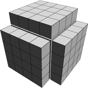
In chapter two, I showed that when we enlarge a square on the side of $a$, we always add $2a+1$ squares to it, and for a big $a$, we can neglect the one, which you can see is that the derivative of the square content of $S=a^2$ (its change) is equal to $2a$. This is in line with the paragraphs above. For clarity's sake, let me show graphically that this is also true in three dimensions. In the higher dimensions, the drawings would already be somewhat complicated.

The constant function is a slightly different cup of coffee, it's $f(x)=C$, where $C$ denotes any number. So for any $x$, the $f(x)$ function returns the same $C$. If we graph a function, we see a straight line. So we feel that the function doesn't change, its derivative should be zero. This can also be substantiated by calculating: $$\frac{\mathrm{d}}{\mathrm{d}x} f(x) = \lim_{h\to 0} \frac{ f(x+h)-f(x)}{h} = \lim_{h\to 0} \frac{ C-C }{h} = 0 \,.$$
Linearity: this word is not widely used by teachers in schools, but it is nevertheless a core concept in physics and similar disciplines. What's linear is straightforward, simple. So Linearity is sought after by scientists by describing a simplified, approximate description of reality. And the derivative is linear. We're saying that the $f(x)$ function is linear if, for each number, $x$ and $y$ are: $$f(x+y)=f(x)+f(y)\,.$$
In addition, for each $x$ number and $C$ constant: $$f(Cx)=Cf(x)\,.$$
You can verify that these rules do indeed apply to the linear function, but not to the quadratic. Miraculously, the derivative itself meets these rules, mathematically written that for every two functions $f(x)$ and $g(x)$ is: $$\frac{\mathrm{d}}{\mathrm{d}x} \left( f(x) + g(x) \right) = \frac{\mathrm{d}}{\mathrm{d}x} f(x) + \frac{\mathrm{d}}{\mathrm{d}x} g(x)\,.$$
Also, for each $f(x)$ function and each $C$ constant: $$\frac{\mathrm{d}}{\mathrm{d}x} \left( C f(x) \right) =C\frac{\mathrm{d}}{\mathrm{d}x} f(x) \,.$$
In other words, the sum derivative is the sum of the derivatives, and we can factor out the constant before the derivative.
The sine and cosine functions are most commonly encountered in triangles and waves. I will intentionally keep their performance poignant, since their deeper explanation would be lengthy and not directly relevant to the subject. We'll still do their derivatives for interested parties. We use two rules. The first are the sum formulas: $$\begin{align*} \sin(x+y)&=\sin(x)\cos(y)+\sin(y)\cos(x)\,,\\ \cos(x+y)&=\cos(x)\cos(y)-\sin(x)\sin(y)\,. \end{align*}$$
In the samples above, we can see how the sine deviates from linearity. The other two rules are: $$\begin{align*} \lim_{h\to 0} \frac{\sin(h)}{h} &=\lim_{h\to 0} \frac{h}{h} 1\,.\\ \lim_{h\to 0} \cos(h) &= 1\,. \end{align*}$$
Results calculated on the Casio fx-991EX calculator, which I consider to be relatively numerically accurate within those on the market.
A little explanation for these limits. The first one indicates that at the start of the function, the sine looks like the linear function $f(x)=x$. You can verify that by looking at the chart, or by entering a few values close to zero in the calculator. E.g. (in radians) $\sin (0.01) \approx 0.009\,998 $ according to my calculator. Now even has a calculator but writes $\sin (0,000\,01) = 0,000\,01$. The second one takes advantage of the fact that $\cos (0) = 1$, we don't even have to make a complex limit transition.
Armed with four equations, we can count, starting with the sine function: $$\begin{align*} \frac{\mathrm{d}}{\mathrm{d}x} f(x) &= \lim_{h\to 0} \frac{ f(x+h)-f(x)}{h} = \lim_{h\to 0} \frac{ \sin(x+h)-\sin(x)}{h} \\&= \lim_{h\to 0} \frac{ \sin(x)\cos(h)+\cos(x)\sin(h)-\sin(x)}{h} \\&= \lim_{h\to 0} \frac{ \sin(x)\cos(h)-\sin(x)}{h} + \cos(x)\frac{\sin(h)}{h} \\ \frac{\mathrm{d}}{\mathrm{d}x} \sin(x)&= 0 + \cos(x) = \cos(x)\,. \end{align*}$$
We have a similar story for the cosine: $$\begin{align*} \frac{\mathrm{d}}{\mathrm{d}x} f(x) &= \lim_{h\to 0} \frac{ f(x+h)-f(x)}{h} = \lim_{h\to 0} \frac{ \cos(x+h)-\cos(x)}{h} \\&= \lim_{h\to 0} \frac{ \cos(x)\cos(h) - \sin(x)\sin(h)-\cos(x)}{h} \\&= \lim_{h\to 0} \frac{ \cos(x)\cos(h) -\cos(x)}{h} - \sin(x)\frac{\sin(h)}{h} \\ \frac{\mathrm{d}}{\mathrm{d}x} \cos(x) &= 0 - \sin(x) = -\sin(x)\,. \end{align*}$$
It is indeed called exponential, not exponential, just as it makes no sense to say potential. Sometimes we also call this function the exponential. We often hear about this function in the media, e.g. films that attempt to imitate scientific parlance. For example, in Professor Sarah Monroe's film Megapiranha, she says that piranhas reproduce exponentially and she means that they multiply very quickly.
By exponential function, we mean $f(x)=e^x$, where $e\approx 2,718$ is a so-called euler number, a constant. This function will be found in many natural phenomena, such as radioactive decay or graft, and we will be interested in some of its properties for the derivative. The first important property is that $e^{a+b}= e^ae^b$, which is a normal amplification property (e.g. $2^4\cdot 2^4=2^8$). So let's just take a straight derivative: $$\frac{\mathrm{d}}{\mathrm{d}x} f(x) = \lim_{h\to 0} \frac{ f(x+h)-f(x)}{h} = \lim_{h\to 0} \frac{ e^{(x+h)}-e^x}{h} = \lim_{h\to 0} e^x\frac{ e^h-1 }{h} \,. $$
But we've hit hard, we have to calculate what the limit of $\frac{ e^h-1 }{h}$ is when $h$ goes to zero. Unfortunately, we can achieve this with some help from outside. The help is to say that the $e$ number is chosen as follows: $$e\equiv \lim_{n\to \infty} \left( 1 + \frac{1}{n} \right)^{n} \,.$$
With this relationship under our belts, we can continue: $$\begin{align*} &\lim_{h\to 0, n\to \infty} \frac{e^h-1}{h} = \lim_{h\to 0, n\to \infty} \frac{\left(1+\frac{1}{n}\right)^{hn}-1}{h}\\ &= \lim_{h\to 0, n\to \infty} \frac{1+\frac{1}{n}{hn} + h^2\cdot (\dots ) -1}{h} = \lim_{h\to 0, n\to \infty} 1 + h (\dots) = 1 \,. \end{align*}$$
In the first edit, we just substituted and used the $(a^b)^c=a^{bc}$ relationship, which can be seen if you write, for example, $(2^2)^3$. In the second modification, we used a similar procedure to that used to derive a general power function, then all we had to do was make a limit transition that shouldn't be complicated by anything. Overall, we found (by producing this result above) that: $$\frac{\mathrm{d}}{\mathrm{d}x} e^x=e^x\,.$$
But that's very strange -- we found a function whose derivative is the same function. This is very useful in solving differential equations. Does any similar property have another function that we know of? Yes, sine and cosine. You just derivatives four times, and we get the same function. We can infer from this that there is some relationship between exponential and goniometric functions. Indeed, it is called the Euler formula, and according to Richard Feynman, it is the most beautiful mathematical equation. A consequence of the similarity is, for example, the relationship that some people have printed on mugs and T-shirts: $$e^{i\pi} + 1 = 0\,.$$
I will not go into the details of this relationship, I will turn the page by reminding that $e^x>0$. As we learned in the last chapter, a positive derivative means a climb. But the second derivative of this function is also positive. Even the third and all the way to infinity. That means the function grows, its growth grows, its growth grows, its growth grows... That's a pretty crazy, really exponential equation that describes turbulent and fast things: an increase in the number of people over time, an increase in the money in the rich people's account, the number of rabbits in the population, the number infected with a dangerous disease, etc.
The logarithm of naturalis, or natural logarithm, is denoted by $f(x)=\ln(x)$. We're writing $y=\ln(x)$ and we mean that $y$ is the kind of number that we have to raise $e$ (the number from the exponential considerations above) to receive $x$. Consider that this is the inverse of $e^x$, so that $\ln (e^x)=x$. To derive a derivative, we will need the following two rules: $$\begin{align*} \ln(a)-\ln(b) &= \ln\left(\frac{a}{b}\right) \,,\\ b\cdot\ln(a) &= \ln (a^b) \,. \end{align*}$$
These are standard rules that apply to the logarithm. You can see both by imagining more specific numbers and recalling the rules $a^b/a^c=a^{b-c}$ and $(a^b)^c=a^{bc}$. Now let's derive: $$\begin{align*} \frac{\mathrm{d}}{\mathrm{d}x} f(x) &= \lim_{h\to 0} \frac{ \ln(x+h)-\ln(x)}{h} = \lim_{h\to 0} \frac{ \ln \left(1 + \frac{h}{x} \right)}{h} \\&= \lim_{h\to 0} \frac{ \ln \left(1 + \frac{h}{x} \right)}{x\frac{h}{x}} = \lim_{h\to 0} \frac{1}{x}\frac{x}{h} \ln \left(1 + \frac{h}{x} \right) \\&= \lim_{h\to 0} \frac{1}{x} \ln \left(1 + \frac{h}{x} \right)^\frac{x}{h} \\ \frac{\mathrm{d}}{\mathrm{d}x} \ln(x) &=\frac{1}{x} \ln (e) = \frac{1}{x}\,. \end{align*}$$
In the second adjustment, we used the first rule for logarithms, in the third one, then we just rewrote the fraction. Now comes a slightly problematic step: adjusting the logarithm. But we can imagine that $h/x = 1/n$, and then for $n\to \infty$, we have the definition of the number $e$. Finally, using $\ln (e) =1$, we revealed the derivative of logarithm.
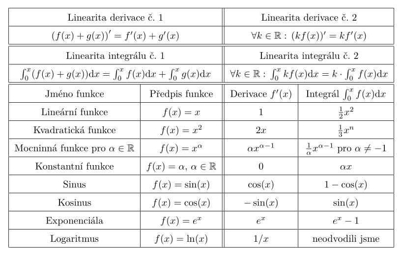
Maybe you're feeling anxious right now because you're wondering how difficult it's going to be to derive all the results for the integrals. But anxiety should be relieved by the basic theorem of differential calculus, which is why we derived it. We do not have to infer integration as laboriously as we did, for example, in the chapter on Archimedes, even if we could. Just use the fact that a derivative is an inverse to integrate. The correct integral can then only be guessed. So the results on the integrals are just summarized in a table, and you can then verify them.
Below is the desired derivative and integration table. You can download it in pdf or look at the source file .tex.
To derive. The linearity of the integral applies, inter alia, for geometric reasons. The area under the function $f(x)+g(x)$ is the same as if we had plotted an area below $f(x)$ on a graph and above it an area below $g(x)$. Equally, the area under the $k\cdot f(x)$ function is only $k$-times the stretched area under the $f(x)$ function.
Now, to verify the accuracy of integration, we have to take the fourth column and get the second column. In the fourth column, there are primitive functions to the original function here. Why are some functions still adding or subtracting some numbers? The point is that to not have numbers, the studied function would have to start at $y=0$. But, for example, for the $e^x$ function, $e^0=1$, this function starts at $y=1$. So the subtracted constant ensures that if we integrate from $a=0$ into $b=0$, we get a zero area under the curve (which itself has a zero length, so that makes sense). The constant does not show up on the control because its derivative is equal to zero.
 About
About Articles
 Tutorials
 External links
 About me